Modeling Market Convergence as Counterflow Heat Exchange

⚠️ This article is for educational, mathematical, and engineering purposes only. It does not constitute financial advice, an investment recommendation, or a trading signal. Cryptocurrency markets are volatile, leveraged markets can fail abruptly, and any implementation must be independently validated before it is used with real capital.

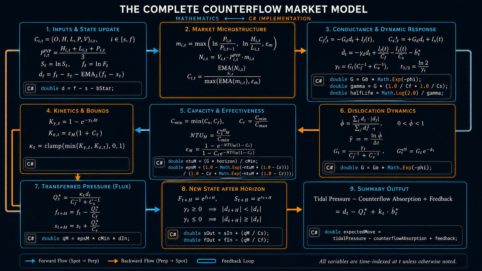
In the Ocean Model, we treated visible price movement as the surface of a much deeper system.

Tides represented observable trend. Underflows represented liquidity, order flow, and liquidation pressure. Storms represented sentiment events capable of transferring sudden energy into the entire market.

But there is another question hiding beneath those layers:

When two connected markets disagree, how much of that disagreement can their available liquidity absorb, how quickly can they absorb it, and which market is likely to move the most?

A counterflow heat exchanger gives us an interesting mathematical language for answering that question.

In a physical exchanger, two fluids travel in opposite directions while transferring heat through a shared boundary. The amount of heat transferred depends on their temperature difference, their heat-capacity rates, the conductance between them, the time available for exchange, and any fouling that obstructs the transfer.

In a crypto market, spot and perpetual futures can also behave like two connected streams.

When a perpetual future trades above its fair relationship to spot, arbitrage pressure may buy spot and short the perpetual. Those actions apply opposing price pressure to the two markets. When the perpetual trades below spot, the flow can reverse.

Markets do not literally obey thermodynamics. They are open, stochastic, reflexive systems filled with new orders, canceled orders, liquidations, funding payments, latency, changing leverage, and human behavior. The purpose of this model is not to claim otherwise.

The useful part is the structure:

• A difference creates pressure.
• Liquidity determines how much pressure each market can absorb.
• Coupling determines how quickly the pressure transfers.
• Friction weakens the transfer.
• A weak stream moves more than a strong stream.
• Under stress, convergence can fail and become amplification.

That gives us the Counterflow Market Model.

The Counterflow Market Model

Heat exchanger concept	Market interpretation	Symbol
Hot stream	The market currently priced above fair relationship	—
Cold stream	The market currently priced below fair relationship	—
Temperature difference	Fair-adjusted spot/perpetual basis
Heat-capacity rate	Candle-derived liquidity or price-impact capacity
Heat-transfer conductance	Cross-market convergence strength
Number of Transfer Units	Coupling relative to the weaker market
Effectiveness	Fraction of maximum transferable pressure
Heat transferred	Model-equivalent transferred notional
Fouling	Fees, latency, borrow limits, margin stress, and venue risk
Outlet states	Forecast spot and perpetual prices after partial convergence

The strongest initial application is a synchronized pair of candles for the same asset:

• One candle from the spot market.
• One candle from the perpetual-futures market.
• The same quote currency or a carefully normalized equivalent.
• The same opening time, closing time, and candle interval.

The model can later be adapted to two exchanges, two related instruments, or the bid and ask sides of a limit order book. Spot versus perpetual futures is simply the cleanest place to begin because the two markets have an explicit economic reason to remain connected.

Now, let’s break this down into its parts, and code!

Standard Candle Inputs

The candle-only implementation uses conventional OHLCV data:

public readonly record struct Candle(  
    DateTimeOffset OpenTime,
    DateTimeOffset CloseTime,
    double Open,
    double High,
    double Low,
    double Close,
    double Volume)
{
    public TimeSpan Duration => CloseTime - OpenTime;
    public double TypicalPrice => (High + Low + Close) / 3.0;
}

The spot and perpetual candles must be synchronized. The model also assumes that volume has been normalized into comparable base-asset units.

That last requirement matters!

Spot volume may already be expressed in BTC, ETH, or another base asset. Perpetual volume may instead be reported as contracts, quote currency, or inverse-contract notional. The model cannot compare those values until the exchange-specific contract definition has been normalized.

A linear contract can often be handled with a contract multiplier:

double baseVolume = candle.Volume * contractMultiplier;  
double quoteNotional = baseVolume * candle.TypicalPrice;  

Inverse and quanto contracts require instrument-specific conversion before entering this model.

The Pressure Difference

Let the logarithmic spot and perpetual states be:

The observed logarithmic basis is:

A raw basis is not automatically a dislocation. Funding, interest-rate differences, borrow costs, collateral demand, and persistent venue structure can support a nonzero relationship between the two prices.

We therefore define a fair basis:

and measure the residual pressure:

When , the perpetual is expensive relative to the estimated fair relationship. When , the perpetual is cheap relative to that relationship.

With only standard candles, we do not have enough information to calculate a full funding-and-carry model. The candle-only implementation therefore uses a slow, causal exponential moving average of the basis:

The current basis is compared against the previous EMA value before the current observation updates it. That prevents the present candle from partially explaining itself.

public sealed class FairBasisEstimator  
{
    private readonly Ema _ema;

    public FairBasisEstimator(int period)
    {
        _ema = new Ema(period);
    }

    public (double Basis, double FairBasis, double Residual) Update(
        double spotClose,
        double perpetualClose)
    {
        double basis = Math.Log(perpetualClose / spotClose);

        if (!_ema.HasValue)
        {
            _ema.Update(basis);
            return (basis, basis, 0.0);
        }

        double fairBasis = _ema.Value;
        double residual = basis - fairBasis;

        _ema.Update(basis);
        return (basis, fairBasis, residual);
    }
}

If funding, interest, and borrow data become available, the external fair-basis estimate should replace the EMA proxy rather than being added on top of it.

For display, a logarithmic ratio can be converted to basis points with:

public static double ToBasisPoints(double logRatio) =>  
    10_000.0 * (Math.Exp(logRatio) - 1.0);

Candle-Derived Liquidity Capacity

A physical heat-capacity rate describes how much energy is required to change a stream’s temperature.

The market equivalent should describe how much notional activity is associated with a unit of price movement.

At order-book resolution, this should be estimated from depth, spread, replenishment, cancellation, and realized price impact. Standard candles do not contain those fields, so we need an observable proxy.

First, calculate effective logarithmic movement:

This combines close-to-close movement with the candle’s intraperiod range.

Next, calculate approximate quote notional:

where converts reported volume into comparable base units.

The candle-derived capacity is then:

A market processing large notional with little movement receives a high capacity. A market moving sharply on modest notional receives a low capacity.

public sealed class CandleCapacityEstimator  
{
    private readonly Ema _notional;
    private readonly Ema _movement;
    private readonly double _minimumMovement;
    private double? _previousClose;

    public CandleCapacityEstimator(int period, double minimumMovement = 1e-6)
    {
        _notional = new Ema(period);
        _movement = new Ema(period);
        _minimumMovement = minimumMovement;
    }

    public double Update(Candle candle, double volumeMultiplier = 1.0)
    {
        double logRange = Math.Log(candle.High / candle.Low);

        double closeMove = _previousClose.HasValue
            ? Math.Abs(Math.Log(candle.Close / _previousClose.Value))
            : logRange;

        double effectiveMovement = Math.Max(
            _minimumMovement,
            Math.Max(logRange, closeMove));

        double quoteNotional = candle.Volume
                             * volumeMultiplier
                             * candle.TypicalPrice;

        double smoothedNotional = _notional.Update(quoteNotional);
        double smoothedMovement = _movement.Update(effectiveMovement);

        _previousClose = candle.Close;

        return smoothedNotional /
               Math.Max(smoothedMovement, _minimumMovement);
    }
}

This is a liquidity proxy, not literal order-book depth. It is still useful because it preserves the important relationship:

More notional with less movement implies greater resistance to transferred pressure.

It also gives the model a capacity with useful units:

Coupled Spot and Perpetual Dynamics

The exchanger analogy becomes clearer when the two markets are written as coupled differential equations:

where:

• is perpetual capacity.
• is spot capacity.
• is cross-market conductance.
• is external perpetual order pressure.
• is external spot order pressure.

When , the coupling term pushes the perpetual downward and spot upward. When , the signs reverse.

The residual basis evolves approximately as:

If external pressure and movement in fair basis are temporarily ignored, the residual has an exponential convergence form:

with:

The solution over horizon is:

and the theoretical half-life is:

The half-life tells us how long the current coupling regime would take to remove half of a dislocation if its estimated behavior remained stable.

Estimating Convergence from Candles

The candle stream can estimate basis persistence with a rolling autoregressive relationship:

Using a no-intercept rolling least-squares estimate:

For monotonic convergence:

and the continuous decay rate is:

public sealed class RollingBasisPersistence  
{
    private readonly Queue<(double Cross, double Square)> _samples = new();
    private readonly int _window;
    private double _sumCross;
    private double _sumSquares;

    public RollingBasisPersistence(int window)
    {
        _window = window;
    }

    public void Add(double previousResidual, double currentResidual)
    {
        var sample = (
            Cross: previousResidual * currentResidual,
            Square: previousResidual * previousResidual);

        _samples.Enqueue(sample);
        _sumCross += sample.Cross;
        _sumSquares += sample.Square;

        while (_samples.Count > _window)
        {
            var removed = _samples.Dequeue();
            _sumCross -= removed.Cross;
            _sumSquares -= removed.Square;
        }
    }

    public (double Phi, double Gamma, TimeSpan? HalfLife) Estimate(
        TimeSpan candleDuration)
    {
        if (_sumSquares <= 1e-24)
            return (double.NaN, 0.0, null);

        double phi = _sumCross / _sumSquares;

        if (phi < 0.0 || phi >= 1.0)
            return (phi, 0.0, null);

        double safePhi = Math.Max(phi, 1e-12);
        double gamma = -Math.Log(safePhi) /
                       candleDuration.TotalSeconds;

        double halfLifeSeconds = Math.Log(2.0) / gamma;

        return (
            phi,
            gamma,
            TimeSpan.FromSeconds(halfLifeSeconds));
    }
}

The value of also identifies the current regime:

Persistence estimate	Interpretation
	Monotonic convergence
	Oscillating convergence or repeated basis crossing
	Little decay or persistent oscillation
	Divergence or amplification

Only the first regime behaves like a passive heat exchanger.

A negative means the basis is crossing its estimated equilibrium while shrinking. A value with magnitude greater than one means the residual is growing. Liquidation cascades, collateral stress, exchange failures, or one-sided directional demand can all produce a market that amplifies pressure instead of absorbing it.

The model should report those regimes rather than forcing every observation into a convergence forecast.

Market Conductance

Once , , and are known, conductance follows directly:

double inverseCapacitySum = (1.0 / perpetualCapacity)  
                          + (1.0 / spotCapacity);

double conductance = gamma > 0.0  
    ? gamma / inverseCapacitySum
    : 0.0;

A high means the markets are strongly coupled relative to the price impact implied by their candles. A low means that basis pressure is transferring slowly.

Market Fouling

Physical fouling adds resistance to a heat exchanger. Market fouling can represent:

• Trading fees and spread.
• Execution latency.
• Borrow scarcity.
• Funding uncertainty.
• Margin requirements.
• Capital fragmentation across venues.
• Withdrawal restrictions.
• Exchange or stablecoin risk.

A convenient scenario penalty is:

double effectiveConductance = historicalConductance  
                            * Math.Exp(-scenarioFouling);

There is an important modeling detail here: a convergence rate estimated from historical candles already contains the friction that was present during those candles.

Therefore, should be the default when describing the observed market. A positive fouling value should be used only for additional scenario analysis or when the conductance estimate comes from a frictionless baseline. Applying historical friction twice would artificially suppress convergence.

Market NTU

The physical Number of Transfer Units is:

For the market model, becomes conductance accumulated over a forecast horizon :

where:

and the capacity ratio is:

A high means that coupling is strong relative to the weaker market’s ability to absorb pressure during the selected horizon. A low means that the two markets may remain disconnected long enough for the dislocation to persist.

double cMin = Math.Min(spotCapacity, perpetualCapacity);  
double cMax = Math.Max(spotCapacity, perpetualCapacity);  
double capacityRatio = cMin / cMax;

double horizonSeconds = candleDuration.TotalSeconds  
                      * forecastHorizonCandles;

double marketNtu = effectiveConductance  
                 * horizonSeconds
                 / cMin;

Counterflow Effectiveness

For a counterflow exchanger, effectiveness is:

When the two capacities are balanced and :

public static double CounterflowEffectiveness(  
    double ntu,
    double capacityRatio)
{
    if (!double.IsFinite(ntu) || ntu <= 0.0)
        return 0.0;

    double cr = Math.Clamp(capacityRatio, 0.0, 1.0);

    if (Math.Abs(1.0 - cr) < 1e-9)
        return Math.Clamp(ntu / (1.0 + ntu), 0.0, 1.0);

    double exponential = Math.Exp(-ntu * (1.0 - cr));
    double denominator = 1.0 - cr * exponential;

    return Math.Clamp(
        (1.0 - exponential) / denominator,
        0.0,
        1.0);
}

Effectiveness is not the probability that a trade succeeds.

It is also not automatically the percentage of basis expected to disappear. It describes transferred pressure relative to the maximum transfer allowed by the weaker-capacity stream.

Transferable Market Pressure

The maximum exchanger-style transfer is:

and the effectiveness-adjusted transfer is:

The resulting fractional reduction in the market gap would be:

Since:

we can also write:

A physical counterflow exchanger can produce outlet states that cross when the exchange is sufficiently effective. Markets can overshoot too, but predicting that crossing from candles alone would be aggressive.

The implementation therefore uses a conservative, bounded closure model.

The empirically observed exponential closure is:

The final forecast closure is the stricter of empirical decay and structural exchanger capacity:

double dynamicClosure = gamma > 0.0  
    ? 1.0 - Math.Exp(-gamma * horizonSeconds)
    : 0.0;

double exchangerClosure = Math.Clamp(  
    effectiveness
    * cMin
    * inverseCapacitySum,
    0.0,
    1.0);

double forecastClosure = Math.Clamp(  
    Math.Min(dynamicClosure, exchangerClosure),
    0.0,
    1.0);

This is deliberately conservative.

The exchanger equations are not allowed to claim more convergence than the recent basis-decay history supports, and the historical decay model is not allowed to claim more pressure transfer than the current capacity relationship supports.

Forecasting the Two Outlet Prices

The bounded model-equivalent transfer notional is:

The forecast logarithmic states are:

Converting back to prices:

double transferNotional = forecastClosure  
                        * residualBasis
                        / inverseCapacitySum;

double spotLogOut = Math.Log(spot.Close)  
                  + transferNotional / spotCapacity;

double perpetualLogOut = Math.Log(perpetual.Close)  
                       - transferNotional / perpetualCapacity;

double predictedSpot = Math.Exp(spotLogOut);  
double predictedPerpetual = Math.Exp(perpetualLogOut);  

The weaker market moves more because the same transferred pressure produces a larger logarithmic price change when divided by a smaller capacity.

If perpetual capacity is much smaller than spot capacity, most of a positive residual basis is expected to close through the perpetual moving downward. If spot capacity is much smaller, more of the adjustment is assigned to spot moving upward.

The value is a model-equivalent notional. It should not be interpreted as proof that an identical quantity of trades will execute during the horizon.

The Complete Candle Loop

The complete implementation maintains:

• A causal fair-basis estimator.
• Separate spot and perpetual capacity estimators.
• A rolling basis-persistence regression.
• A rolling residual z-score.
• Regime classification.
• Conductance, NTU, effectiveness, closure, transfer, and outlet forecasts.

A typical configuration for 15-minute candles might begin with:

var model = new CounterflowMarketModel(  
    new CounterflowParameters
    {
        FairBasisPeriod = 96,          // About one day
        CapacityPeriod = 32,           // About eight hours
        ConvergenceWindow = 128,       // About thirty-two hours
        MinimumConvergenceSamples = 32,
        ResidualZScoreWindow = 128,
        ForecastHorizonCandles = 4,    // One-hour horizon
        SpotVolumeMultiplier = 1.0,
        PerpetualVolumeMultiplier = 1.0
    });

The model is updated once for each synchronized candle pair:

foreach ((Candle spot, Candle perpetual) in alignedCandles)  
{
    CounterflowSnapshot state = model.Update(
        spot,
        perpetual,
        externalFairLogBasis: null,
        scenarioFouling: 0.0);

    if (!state.IsReady)
        continue;

    Console.WriteLine(
        $"{state.Time:u} " +
        $"Regime={state.Regime} " +
        $"Residual={state.ResidualBasisBps:F2}bps " +
        $"Z={state.ResidualZScore:F2} " +
        $"Phi={state.Phi:F4} " +
        $"HalfLife={state.HalfLife} " +
        $"NTU={state.MarketNtu:F4} " +
        $"Effectiveness={state.Effectiveness:P2} " +
        $"Closure={state.ForecastClosureFraction:P2} " +
        $"SpotOut={state.PredictedSpotClose:F2} " +
        $"PerpOut={state.PredictedPerpetualClose:F2}");
}

The full dependency-free .NET implementation accompanying this article includes validation and all helper classes in one source file.

Reading the Output

A positive residual does not mean that spot must rise, nor does it mean that the perpetual must fall.

It means that the pair is above its estimated fair basis. Capacity determines how the modeled adjustment is divided between the two markets. New directional pressure can still move both prices upward or downward while the basis closes between them.

That is an important distinction:

The Counterflow Market Model forecasts relative convergence, not the absolute direction of the entire crypto market.

Where the Model Breaks

A physical exchanger is passive. A market is not.

New information can enter at any moment. Traders can withdraw liquidity. Liquidations can force execution. Funding can change. Exchanges can become unavailable. A price gap can attract arbitrage capital, but that same gap can also signal genuine credit, collateral, or venue risk.

Standard candles create additional limitations:

• They do not reveal the bid–ask spread.
• They do not reveal order-book depth.
• They do not distinguish market orders from limit orders.
• They do not expose cancellation or replenishment rates.
• They do not contain funding, open interest, liquidations, borrow rates, or latency.
• Reported volume may be distorted or incomparable across venues.
• A candle close hides the path taken inside the interval.

The candle-derived capacities are therefore empirical proxies. They should be replaced with direct impact curves when full market microstructure data is available.

A production study should also use:

• Walk-forward rather than full-history calibration.
• Strictly causal feature construction.
• Exchange-specific volume normalization.
• Robust outlier handling.
• Fee, spread, slippage, and funding simulation.
• Separate validation across calm, trending, and liquidation regimes.
• Mark-price, index-price, and traded-price comparisons.
• Venue-failure and stale-data detection.

The most dangerous regime is amplification.

When , the residual magnitude is growing instead of decaying. For , the first-order differential equivalent has negative damping:

A value represents a growing sign-alternating process and cannot be represented by the simple monotonic exchanger equation at all. In either case, the heat-exchanger analogy is no longer the right local model. The system is behaving more like a feedback amplifier or runaway reaction. The implementation correctly reports divergence and suppresses the passive-convergence forecast.

Adding Counterflow to the Ocean Model

The Counterflow Market Model fits naturally beneath the Ocean Model as a microstructure absorption layer.

The Ocean Model asks:

• What direction is market energy moving?
• How are surface trend, underflow pressure, liquidation heat, and sentiment coupled?

The Counterflow Model asks:

• How much relative pressure can connected liquidity absorb?
• How quickly should a dislocation decay?
• Which market is structurally weaker?
• Is the pair converging, oscillating, or amplifying?

The combined interpretation becomes:

The Ocean Model can provide directional force. Counterflow can provide resistance, transfer capacity, and timing.

For example, a strong bullish surface and underflow state may still produce very different outcomes:

• High spot capacity and low perpetual capacity can push most relative adjustment into the perpetual.
• Low capacity on both streams can turn modest order pressure into large price movement.
• High NTU with a short half-life suggests that temporary basis dislocations should be absorbed quickly.
• Low NTU suggests that the markets are weakly coupled and the basis may persist.
• A divergent persistence estimate warns that liquidations or structural stress may be overwhelming ordinary arbitrage.

This gives the broader model something it did not previously have: a mathematically explicit estimate of how much incoming pressure the connected market structure can absorb before that pressure becomes visible movement.

The Exchanging Market

A counterflow heat exchanger does not predict where heat originated. It predicts how two streams exchange energy once a difference exists.

The Counterflow Market Model should be understood the same way.

It does not primarily answer:

Will Bitcoin go up?

It answers a narrower and more mechanically useful set of questions:

How large is the current spot–perpetual dislocation after fair basis is removed?

How much resistance does each market appear to have?

How strongly are the two markets coupled?

How much of the dislocation can plausibly transfer during the selected horizon?

Which market is likely to perform most of the relative adjustment?

Is the system absorbing pressure—or amplifying it?

That makes the model testable.

Each state can be calculated from synchronized candles. Each parameter can be measured walk-forward. Each forecast can be compared with the observed future basis and the realized contribution of spot and perpetual price movement.

The analogy provides the architecture.

The market data must determine whether the architecture is useful!

Engineering References

1. Damien Ackerer, Julien Hugonnier, and Urban Jermann, Perpetual Futures Pricing, arXiv:2310.11771.
2. Songrun He, Asaf Manela, Omri Ross, and Victor von Wachter, Fundamentals of Perpetual Futures, arXiv:2212.06888.
3. Rama Cont, Arseniy Kukanov, and Sasha Stoikov, The Price Impact of Order Book Events, arXiv:1011.6402.
4. NPTEL, Heat Exchangers, Module 7, Effectiveness–NTU Method.